This week you’ll first install and set up MARS. Then, you’ll learn some of the basic things in MIPS that you’ll need for many programs in the future, such as:
- how to print out numbers, newlines, and strings
- how to get numeric and string input from the user
- how to do simple computations
Try this: boxes labeled “try this” are things to play around with and learn a little more. They are not required and you don’t have to turn in the code you write for these, so you can erase that code when you’re done playing around.
1. Getting and installing MARS
You must use my modified version of MARS! Not the one from Missouri State! Don’t just google MARS! Cmon!
Go to the Software page and download the version of MARS appropriate for your computer.
Platform-specific instructions follow:
Windows users
If you have a previous version of MARS installed, first you need to uninstall it. Start, type “add remove”, run “Add or Remove Programs,” search for MARS, click the three dots on the right, and uninstall. No, this will not delete any of your data.
- Run the
.exefile you downloaded. If it whines about it being “unverified” or whatever:- click “More”
- click “Run Anyway”
- It will install MARS. That’s all it does. It might not even seem like anything happened, but no news is good news.
- Then open the Start menu and run it.
- It might be on the “recently installed” list, or you can type “mars” to find it.
That should be it.
macOS (Apple) users
If you have a previous version of MARS installed, first you need to uninstall it. Open Finder, Go > Applications, look for Mars, and then delete it (select it, ⌘delete, or drag to recycle bin). No, this will not delete any of your data.
- Run the
.dmgfile you downloaded. - Drag the MARS icon into the Applications folder.
- Eject the
.dmgfile. (Ask for help if you don’t know how)
Now, you have to tell macOS to let you run the program. You only have to do this the first time you run MARS:
- Go into your Applications folder.
- Right-click the MARS icon, and click Open.
- Click “Open Anyway” or whatever it says.
- On newer versions of macOS, this will not work. Instead:
- Open System Preferences
- Go to Privacy & Security
- Scroll down until you see the message
"Mars_2254_0111" was blocked from use because it is not from an identified developer.", and click Open Anyway. - Then it’ll ask for your password/fingerprint…
- …and then ask you to click Open Anyway, and then it’ll work.
From now on, you can just run it normally (e.g. pin it to the dock, or ⌘Space, type mars, hit enter)
Linux Users (including Chromebooks!)
You need to have a modern Java runtime environment installed. I think Java 11 is the oldest version that MARS will work with, but even that’s pretty old by now. Check with java -version.
You can run the jar file from the shell like:
java -jar Mars_2254_0111.jar
Or maybe you can just double-click it? idk
2. Hello, nothing
It is crucial that you get this section working before moving on. This is the most fundamental thing for doing work in this course. If you have any problems with this section, you need to ask me (or a TA, once we know who they are) for help immediately. I’m not kidding.
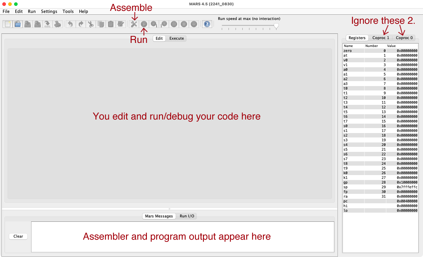
When you run MARS, it looks something like this:
Setting things up (important!)
In the Settings menu, make sure the following things are checked (enabled):
- ✔ Show Labels Window (symbol table)
- ✔ Clear Run I/O upon assembling
- ✔ Initialize Program Counter to global ‘main’ if defined
Leave the other settings unchanged.
Also, if the “Mars Messages” at the bottom is huge, drag the white horizontal divider above it down.
Now:
- File > New
- In MIPS, comments start with a
#sign. At the top of the file, put your full name and username in a comment. -
Just like in Java or C, our assembly programs start at a
mainfunction. Type, don’t copy, these lines into your file.The
.globaldirective is only needed formain. None of your other functions need it..global main main:main:is a label. Labels name parts of your code; not just functions, but also loops, if-elses, variables, etc. - At this point, you cannot hit the
 assemble button. That’s because you haven’t saved.
- Hit Ctrl+S/⌘S. This brings up the save dialog.
- Name the file
abc123_lab4.asmwhereabc123is your username. (e.g. I’d name minejfb42_lab4.asm) - Navigate into your personal files:
- Windows: your files are in
C:\Users\<your username>. Desktop and Documents are in there. - macOS: your files are in
/Users/<your username>Desktop and Documents are in there. - Linux: your files are in
/home/<your username>but you probably knew that.
- Windows: your files are in
- Finally hit the save button.
- If you get an error with
FileNotFoundExceptionand (Read-only file system), you’re trying to save somewhere other than your personal files. Look at the previous step.
- If you get an error with
-
Instead of “compiling,” we “assemble” an asm program. When you assemble the program with the
assemble button, it’ll switch to the Execute tab.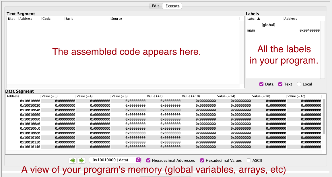
-
Now run with
 . In the “Run I/O” at the bottom of the screen, it’ll say
-- program is finished running (dropped off bottom) --It’s a completely empty program that does nothing. Yay!
Try this: what error do you get if you remove the .global main line? Well now you know what to do if you see that error. :)
3. Playing with registers
Now you’ll learn how to put integers into registers and copy them around, and also to step through your program one instruction at a time.
Registers are like the CPU’s hands. Each one can contain a 32-bit value. What that value means or is is up to us, the programmers.
In Java, we have variables. We can put values into variables and copy values from one variable to another. There are analogous operations on registers in asm, but it’s not as straightforward as the = operator in Java.
Look at the register pane on the right side of the window. There are 35 registers listed, and all but gp, sp, and pc contain 0 (shown by default in hexadecimal as 0x00000000).. These are the values they are set to when your program starts.
“Immediate” means “a constant that is embedded within the instruction.”
-
Type, don’t copy, these instructions after your
main:line.listands for “load immediate”, and it puts a constant value into a register.li t0, 1 li t1, 2 li t2, 3By analogy to Java,
li t0, 1is like doingt0 = 1. - Assemble and run. Those
t0, t1, t2registers on the right side changed to 1, 2, and 3!- You may have to uncheck “Hexadecimal Values” at the bottom of the Data Segment view on the Execute tab for the values to be more readable.
-
But it was too fast to see what happened. Assemble again, but this time, step through instruction-by-instruction with the
 step button. Watch the values of the registers and the highlighted instruction in the text window.
- You’ll see the registers highlighted green when they change.
- You’ll notice that the highlighted instruction is the one that is just about to run. This trips a lot of people up! The effects of the instruction will not take place until you execute that instruction and move onto the next one.
-
But wait! You can go backwards too. Use this button:
 .
.- You’ll see the instructions happen in reverse, and the registers will get set back to 0.
Stepping forward and backward one instruction at a time is extremely helpful when you first learn to program assembly. (It’s extremely helpful even when you’ve been using it for years, too.)
Half a century ago, someone decided to use the word “move” instead of “copy” and now we’re stuck with it. Sorry!
-
Last, we can copy values between registers with the
moveinstruction. After yourlis, write these lines:move a0, t0 move v0, t1 move t2, zero- Assemble and step through. The values are copied from the register on the right into the register on the left. This is important: data is never “moved” on a computer, always copied. (What would moving it even do? What would be left in the original register? I dunno.)
A really, really common mistake is to read
move a0, t0as “movea0intot0”. This is backwards. Try to imaginemove a0, t0asa0 = t0instead.
Try this: Load a hexadecimal immediate into a register, like li t0, 0xF00D. Assemble, and look at the “Code” column in the text segment. Do you see it?
Now try putting a value into the zero register. That’s its name. li zero, 10. What happens when that runs? What value is still in it? Why do you think the register is named zero then? ;o
When you step through your program, one other register changes on every instruction… step back, too. What register is that? What do you notice about its value? With “Hexadecimal Values” on, do you see its values anywhere else in the execute tab?
Errors and line numbers
A lot of newer programmers seem to think that when they get errors (either compiler/assembler errors or runtime errors), they just have to guess and infer where the error happens. Not true! Pretty much every error message you ever get in Java or MIPS tells you exactly where in your code the error is.
-
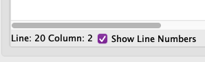
At the bottom left of the code editor in MARS, make sure this “Show Line Numbers” checkbox is checked (there is no reason to ever uncheck it):
-
Let’s introduce an error into our program to test this out. In the code you just wrote, change one of the
moves toli. (Like, changemove a0, t0toli a0, t0.) Now assemble. -
You’ll see an error at the bottom in the “Mars Messages” panel that looks something like this:
Error in /path/to/your/abc123_lab4.asm line 16 column 9: "t0": operand is of incorrect type (expected INTEGER_16, got REGISTER_NAME)- See, there is no need to guess what part of your code is causing the problem. It says it’s on line 16 in your
_lab4.asmfile. - Then, if you double-click that error message, it takes you to that line of your code and highlights it!
- See, there is no need to guess what part of your code is causing the problem. It says it’s on line 16 in your
-
Change that code back so it works again.
Code formatting
This applies to any language, not just assembly: do not treat code formatting as a “final step” you do to “clean things up” before submitting. It is not. Code formatting is absolutely crucial for making your code readable and understandable. Keep your code formatted nicely while you write it, not at the end.
Those of you who are already getting reliant on the “format source code” tool in VS Code: stop 😤
Go to the Materials page and look for the “MIPS style guide” in the References. Have a look at the code comparisons in particular. Here is an important rule about dealing with indentation, in any programming language:
Never use the spacebar at the beginning of a line of code to “line things up.” That is what the Tab key is for.
Go ahead. Try using the spacebar to indent your code in MARS right now. I dare you. ;)
The Tab key is what you use to indent code. You can also deindent code with Shift+Tab. Finally, you can select several lines of code and use Tab and Shift+Tab to indent and deindent them in virtually any code editor, including MARS.
Knowing all this, format and comment the code you’ve written so far so that it looks like this:
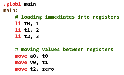
I have my editor settings (Settings > Editor) set a little different from the defaults. If your colors are different or your tabs are wider than the screenshot, that’s fine. Consistency and neatness are the most important parts of code formatting.
4. Printing integers
Now let’s print some integers. (Strings are a little more advanced.)
-
After the previous code, type this (and remember to keep the indentation nice):
# print 123 li a0, 123 li v0, 1 syscall -
Assemble and run, and you’ll see the number
123printed in the “Run I/O”.
What’s going on here? What is a0? What is v0? What is syscall?
As you’ll find out in 449, programs have to ask the operating system to get input or produce output, and we do that with system calls. MARS pretends like it’s a tiny operating system, so it has many built-in system calls to print things out, ask the user to type something, etc.
We choose which system call to run by putting a number into the v0 register before executing the syscall instruction.
From now on, I want you to treat the li v0, whatever and syscall as two halves of the same thing. You do not put any code between the li v0, whatever and the syscall. They go together. Never use syscall without first doing li v0, whatever.
In MARS, go to the “Help > Help” menu item. Then click “Syscalls” on the lower set of tabs. This tells you about what syscalls are, which ones are available, what their numbers are, and their arguments and return values.
Notice it says this at the top of the table:
| Service | Code in $v0 |
Arguments | Result |
|---|---|---|---|
| print integer | 1 | $a0 = integer to print |
There are lots of other possible values you can put into v0 to choose different syscalls, but syscall 1 means “print an integer.”
Then, the arguments to the syscalls go in the a registers. That’s why they are named a0, a1, etc. a is for argument.
So to sum up: the three lines above correspond roughly to this Java code:
System.out.print(123);
5. Printing more integers and newlines
Right now, your program just prints out 123. Now:
- Add code to do the equivalent of
System.out.print(456)after the first print. (It will be another 3 lines.)- Don’t forget to comment your code so you can tell what it does! Write something like
# print(123)before the first set of lines, and something similar for the second set.
- Don’t forget to comment your code so you can tell what it does! Write something like
- Run it and look at the output.
It comes out as 123456. Well, that’s confusing! But that’s because you printed both numbers on the same line. Unfortunately there is no equivalent of System.out.println. So, we have to print the newline ourselves.
- Between the two prints (right after the first
syscall), we are going to do another syscall:- for the argument
a0, use'\n'(that’s single quotes around a backslash andn) - for the syscall number
v0, use11(look up what syscall11does in the MARS help)
- for the argument
- Run it again.
You should now have 123 and then 456 on another line after it. Nice!
6. Integer input and math
Syscall 5 works a bit like Scanner.nextInt() in Java. It:
- waits for the user to type an integer into the “Run I/O” box at the bottom and hit enter,
- parses what the user typed as an int, and
- returns that integer in
v0(because that’s whatv0is for: return values).
- After all the code you’ve written so far, do this:
- print another newline with syscall 11 like you did before (you can copy and paste those lines)
- Use syscall number 5. It takes no arguments, so you don’t have to put anything in the
a0register before using it.
- Run your program, and now instead of stopping, it shows:
 123
 456
 |
with a flashing cursor on the line after
456, which is it waiting for you to type something. - Click on the “Run I/O” box, type a number, and hit enter. The program will end.
- Look at the contents of the
v0register on the right – it should hold the value that you typed in.
If you type something other than a number and hit enter, or hit enter without typing anything, you’ll get something like Runtime exception at 0x00400034: invalid integer input (syscall 5). That’s okay, that’s not a bug or anything. It’s just that syscall 5 is picky and you have to type an integer.
Well if we can now get integers from the user, let’s do something with them. Let’s ask the user for two numbers, add them together, and print the sum.
Right now, at the end of main, v0 contains the number that the user typed in. We want to ask the user for another number, so you have to do syscall 5 again.
But wait. In order to do syscall 5, you have to set v0 to 5. That will destroy the first number that the user just typed in, right?
So you need to put that number somewhere SSSSSssssSSSSSSSSSSsssssafe. I sound like a snake because I’m talking about the s registers. They’re useful for saving values for later.
- After that syscall 5, put the value that the user typed in into
s0.- it’s not
move v0, s0. That’s backwards.
- it’s not
- Then do syscall 5 a second time.
- At this point, you have the two values you want to add together in
s0andv0.- Go to Help > Help, and near the top of the “Basic Instructions” list, you’ll see
add $t1, $t2, $t3.- That’s not literally what you type in though. You can use any registers in place of
$t1, $t2,and$t3. - Read the description of the instruction and see what order things go in.
- That’s not literally what you type in though. You can use any registers in place of
- You want to add those two values together and then print out the sum with syscall 1, so… which register should the sum go into so that you can print it out?
- Go to Help > Help, and near the top of the “Basic Instructions” list, you’ll see
- Finally, after the
addline, do syscall 1 again to print out the sum.
When done correctly, your program should ask for two numbers, then print out their sum, like:
123
456
1000
533
1533
-- program is finished running (dropped off bottom) --
7. Printing strings
Now we can work on printing an actual “hello world” message.
What are strings, anyway?
The first 128 characters of Unicode are ASCII, so technically any ASCII string is also Unicode.
Strings are arrays of characters, and each character is really a number with an agreed-upon meaning. That “agreement” is called a character encoding and says things like “the number 97 means lowercase a.” The most widespread encoding today is Unicode, but there is an older encoding called ASCII which many programs in the English-speaking world use. Go have a look at this table, paying attention to the Dec and Chr columns.
This means that "abc" is really an array of 3 numbers: {97, 98, 99}. But you also need to know how long the string is, or at least where the end of it is. The convention in both the C language and MARS is to use a zero terminator: a character with the value 0 at the end of the string. That means "abc" is represented like this in memory (shown in hexadecimal):
0x61 |
0x62 |
0x63 |
0x00 |
In ASCII, each character - that is, each number - is one Byte. (That’s how many bits?)
Can you put a string in a register?
I said earlier that registers are like the CPU’s hands. Just like your hands, they’re limited in size. You can’t fit a car in your hands. But you can use your hands to point to a car. 👉🚗 You can use registers to point to something too.
Strings are arrays, and arrays are too big to fit in reigsters. Instead, we can only put the address of a string in a register. The address is where the string is located in memory, and it is a 32-bit number in the version of MIPS that we’re using. Conveniently, our registers are 32 bits too!
So no, you can’t put a string in a register, but you can put a string’s address in one.
Hello world at last
In Java, you can just write strings anywhere you like, and the compiler takes care of all of that crap for you. But in asm, we have to be a little more… literal.
Did you just scroll down to this and skip all the stuff above? Of course you didn’t! You totally read all the stuff I wrote above. All that information I could definitely ask about on an exam. Yep. You read it!
- Before your
.global mainline:- Add a
.dataline. This tells the assembler, “switch to the data segment.”- The data segment is the part of memory where we put… data. Variables, strings, etc.
- After that line, write this:
hello_msg: .asciiz "hello, world!\n".asciizsays, “encode the following string asascii, with azero terminator.”- You know what
\ndoes, right?
- After that line, put a
.textline. This tells the assembler, “switch to the text segment.”- The text segment is where code goes.
- Add a
- In
mainat the start of your program (that is, right aftermain:before the code you wrote previously):- Write
la a0, hello_msglastands forloadaddress. It puts the address of a label into a register.- So, this will put the address of
hello_msgintoa0.
- Then, do syscall 4.
- Write
- Assemble and run.
-
Now the first thing it prints should be your “hello, world!” message, before printing and asking for numbers. So it should look like this (ofc what you type in for the numbers is up to you):
hello, world! 123 456 10 20 30 -- program is finished running (dropped off bottom) -- -
You can also assemble and step one instruction at a time - if you turn on “Hexidecimal Values”, you can see the address
0x10010000get put intoa0.
-
Try this: what error do you get if you comment out the .text line? Well now you know what to do if you see that error. :) Similarly, try commenting out the .data line. Those directives are easy to forget.
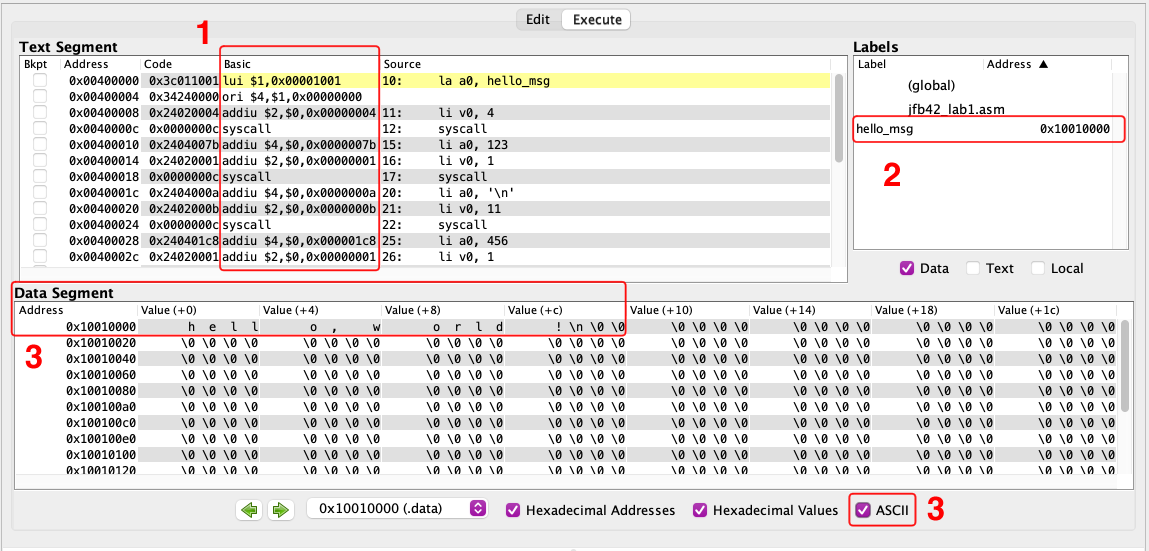
A few things to notice
While you are on the Execute tab, there are three things I want you to look at:
- In the Text Segment panel at the top, you can see the instructions that you wrote, but you can also see the “Basic” column looks a little different.
- If you can’t see the instructions in the Text Segment panel… make MARS wider. Lol.
- Both
laandliare pseudoinstructions: “fake” instructions that the assembler accepts and rewrites to simpler instructions that a MIPS CPU can actually understand. lais rewritten to two instructions,luiandori. It’s fine. Sometimes that happens.
- In the Labels panel, you should see one entry:
hello_msg 0x10010000- That
0x10010000is the memory address that the assembler gave to thehello_msgstring. - Memory addresses are virtually always displayed in hexadecimal.
- That
- If you check the
ASCIIbox at the bottom of the Data Segment panel, you can see your string at the top-left!- You can see
0x10010000- the address - on the left side. - You can also see that after the end of the string is
\0- that’s the zero terminator. (There are many more\0bytes in memory after it, but that one was put there on purpose by the assembler.)
- You can see
8. String input
Now we’ll have the user type in their name and greet them. Real CS 0007 stuff. You are going to change your program so that the input/output look like this instead of just saying “hello, world!”
enter your name: Jarrett
hello, Jarrett
123
456
5
7
12
-- program is finished running (dropped off bottom) --
So you need to replace your current code that prints "hello, world!\n" with:
- Print
"enter your name: ". - Read a string from the user (explained below).
- Print
"hello, "- (there’s no string concatenation so we have to print out each part of this line separately.)
- Print the string they typed in on step 2.
Reading a string from the user
In Java, you would use Scanner.nextLine() which returns a string, but “returning a string” is kind of complicated in a low-level language. So instead, the way this works is, you make space for a string, then you tell the syscall where that space is, and it will put what the user typed in that space.
So to read a string from the user:
- In the
.datasegment, make space for a string by doing something likeinput_buffer: .space 50.- This sets aside 50 bytes starting at
input_buffer. - This could hold a string up to 49 characters long + the zero terminator character.
- This sets aside 50 bytes starting at
- Use syscall 8 to read into the string. It takes two arguments:
a0is the address ofinput_buffer. (laagain)a1is the length of the input buffer. (50 in this case)- Remember that you have to put these things in the
a0anda1registers before doing theli v0, 8andsyscall!
- After the
syscallline, what the user typed will be ininput_buffer.
So to later print out what they typed in… just use syscall 4 with the address of input_buffer as the first argument.
9. Exiting gracefully
Finally, you’ll learn how to exit your program more “properly”.
At the end of your main function (so, the end of your program), use the exit syscall (number 10). It takes no arguments, so you don’t have to put anything in the a0 register.
When you run now, your output should now look something like this (depending on what you type in for the numbers to add):
enter your name: Jarrett
hello, Jarrett
123
456
11
22
33
-- program is finished running --
So, the final message changed to no longer say “dropped off bottom.” It might not seem that important now, but it’ll save you a lot of trouble later if you end every main function with the exit syscall.
Submitting
Upload to Gradescope, once it’s open.
The last submission you upload is the one we grade.