Try to do each one without looking at the solution. If you’re stumped, look at the solution and read the notes that I put in there as well. I try to explain why I solved it that way.
Table of contents, by lecture
- Lecture 2
- Lab 1
- Lecture 3
- Lecture 4
- Lecture 5
- Lecture 6
- Lecture 7
- Lecture 8
- cutoff for exam 1
- Lecture 9
- Lecture 11
- Lecture 13
- Lecture 14
- Lecture 15
- Lecture 16
- Lecture 17
- Lecture 18
- Lecture 21
- Lecture 22
- Lecture 23
Boolean Logic to Gates (Lecture 2)
For each Boolean logic function, draw a small circuit out of gates which implements it. Y is the name of the output, and the other letters are the inputs. These functions use the first-order logic symbols, which are:
- ¬ for NOT
- ∧ for AND
- ∨ for OR
- ⊕ for XOR (exclusive OR)
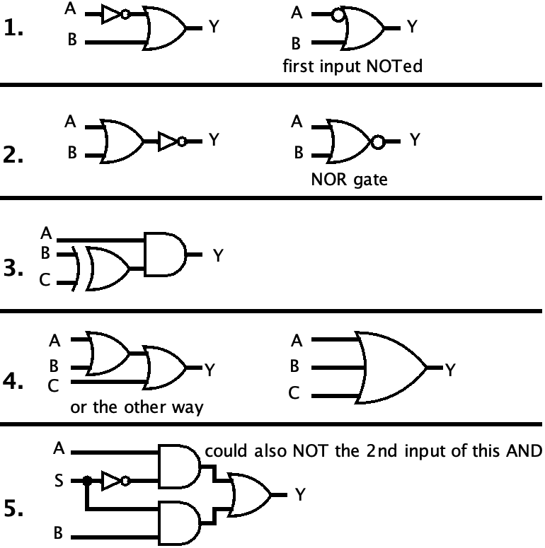
- Y = ¬A ∨ B (order of operations: NOT happens before OR)
- Y = ¬(A ∨ B) (different order now…)
- Y = A ∧ (B ⊕ C)
- Y = A ∨ B ∨ C (I can think of a few ways of drawing this)
- Y = (¬S ∧ A) ∨ (S ∧ B) (S is a single input, so don’t draw it twice)
Sometimes there are multiple ways of drawing certain circuits. I’ve tried to include all options where possible.
Gates to Boolean Logic (Lecture 2)
For each circuit, write the Boolean Logic formula that describes it. Your formulas will all be of the form Y = ....
You can use any convention you like, but be consistent. You can also use parentheses if needed or for clarity. The three conventions are as follows, showing NOT, AND, OR, and XOR respectively:
- First-order logic: ¬A, A∧B, A∨B, A⊕B
- C-style bitwise:
~A, A&B, A|B, A^B(yes,^is bitwise XOR in C and Java, not exponentiation!) - Engineering style: A̅, AB, A+B, A⊕B
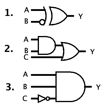
- “Y = A XOR (NOT B)”, or in all three conventions:
- Y = A ⊕ ¬B
- Y = A ^ ~B
- Y = A ⊕ B̅
- “Y = (A AND B) OR C”, or in all three conventions:
- Y = (A ∧ B) ∨ C
- Y = (A & B) | C
- Y = AB + C (in this convention, AND is done before OR so no parentheses needed)
- “Y = A AND B AND (NOT C)”, or in all three conventions:
- Y = A ∧ B ∧ ¬C
- Y = A & B & ~C
- Y = ABC̅ (see how short this is? I think this is why engineers like it…)
The Simple Boolean Function Method (Lab 1)
Use the simple method for turning a truth table into a boolean function that you learned on lab 5. (Find rows where the output is 1, then make an AND term for each row, then OR them together.)
Your answer will look like Y = ..., since the output’s name is Y.
| A | B | C | Y |
|---|---|---|---|
| 0 | 0 | 0 | 0 |
| 0 | 0 | 1 | 1 |
| 0 | 1 | 0 | 0 |
| 0 | 1 | 1 | 0 |
| 1 | 0 | 0 | 1 |
| 1 | 0 | 1 | 0 |
| 1 | 1 | 0 | 1 |
| 1 | 1 | 1 | 0 |
Here are the terms. There should be bars over some of the letters. If they’re not showing up correctly, I’ve also included an English description of the term so you can check your interpretation.
| A | B | C | Y | term | How to read it |
|---|---|---|---|---|---|
| 0 | 0 | 0 | 0 | ||
| 0 | 0 | 1 | 1 | A̅B̅C |
“NOT A and NOT B and C” |
| 0 | 1 | 0 | 0 | ||
| 0 | 1 | 1 | 0 | ||
| 1 | 0 | 0 | 1 | AB̅C̅ |
“A and NOT B and NOT C” |
| 1 | 0 | 1 | 0 | ||
| 1 | 1 | 0 | 1 | ABC̅ |
“A and B and NOT C” |
| 1 | 1 | 1 | 0 |
The final expression: Y = A̅B̅C + AB̅C̅ + ABC̅
Conversion between binary and decimal (Lecture 3)
You may want to practice your powers of two with this page first, just the ones up to 28.
Without using a calculator, convert these binary numbers to decimal. The spaces are just for digit grouping to make the numbers easier to read.
0000 01100000 10010000 11110010 01110101 00000111 1111
Again without using a calculator, convert these decimal numbers to 8-bit binary numbers. Remember: you can always put 0s in front of a number without changing its value.
- 3
- 13
- 26
- 55
- 89
- 104
Binary to decimal:
0000 0110= 60000 1001= 90000 1111= 150010 0111= 390101 0000= 800111 1111= 127
Decimal to binary:
- 3 =
0000 0011 - 13 =
0000 1101 - 26 =
0001 1010 - 55 =
0011 0111 - 89 =
0101 1001 - 104 =
0110 1000
Conversion between binary and hex (Lecture 3)
Without using a calculator, convert these binary numbers to hexadecimal. (Do you remember which end to start grouping the bits from?)
111010110001001111100010011001100100001010011010100111000100110
Again without using a calculator, convert these hexadecimal numbers to binary numbers.
0x550xFFF0xC01B0x287D90xE315BAD(was it ever good?)0xC0000005(wonder if any windows users have seen this number before)
Binary to hex:
11=0x3(not0xC; don’t put0s on the right side of the number!)10101=0x15(not0xA8; you get the idea)10001001=0x8911110001001=0x78910011001000010=0x264210011010100111000100110=0x4D4E26
Hex to binary:
0x55=0101 01010xFFF=1111 1111 11110xC01B=1100 0000 0001 10110x287D9=0010 1000 0111 1101 10010xE315BAD=1110 0011 0001 0101 1011 1010 11010xC0000005=1100 0000 0000 0000 0000 0000 0000 0101
Signed Integers (2’s Complement) (Lecture 4)
Interpret these bit patterns as 8-bit signed integers by converting them to decimal. Write the sign (+ or -).
0000 01100101 10100111 11111000 00011100 11101111 1111
Keep in mind: this is not sign-magnitude. Sign-magnitude is never used with integers anymore. If you interpret the 4th number as “-1”, that’s sign-magnitude and it’s wrong.
Recall that in 2’s complement, the MSB place has a negative value. Here, it’s the -128s place. So if that place is 0, it’s positive; and if it’s 1, you start at -128 and add the value of the rest of the places onto it.
0000 0110= +60101 1010= +900111 1111= +1271000 0001= -1271100 1110= -501111 1111= -1
Ranges of integers (Lecture 4… and 3)
Compute the unsigned and signed ranges of integers with the given numbers of bits. (When I say “compute,” I mean write out the actual values, instead of writing them like 2n or whatever.)
- 3 bits
- 5 bits
- 6 bits
- 8 bits
- 10 bits
- 12 bits
Remember, for signed numbers, there is one more negative than positives. (For signed numbers, the minimum value will always be exactly a power of two, but negative.)
- 3 bits
- unsigned: 0 to 7
- signed: -4 to 3
- 5 bits
- unsigned: 0 to 31
- signed: -16 to 15
- 6 bits
- unsigned: 0 to 63
- signed: -32 to 31
- 8 bits
- unsigned: 0 to 255
- signed: -128 to 127
- 10 bits
- unsigned: 0 to 1023
- signed: -512 to 511
- 12 bits
- unsigned: 0 to 4095
- signed: -2048 to 2047
Binary addition (Lecture 5)
For each pair of numbers:
- calculate the sum by hand.
- convert the two addends (inputs) and sum to unsigned decimal, to check your work.
0001 0110 + 0000 11110011 0011 + 0101 0010
1.
    11 11
  0001 0110 = 22
+ 0000 1111 = 15
-----------
  0010 0101 = 37
2.
  111   1
  0011 0011 = 51
+ 0101 0010 = 82
-----------
  1000 0101 = 133
Detecting overflow (Lecture 6)
Important: computers are dumb as hell and do not understand things like “rules of mathematics” and therefore cannot look at an answer and say “that looks wrong.” All they can do is look at bits (1s and 0s) and tell you if those bits satisfy certain conditions. How a computer detects overflow is extremely simplistic.
We learned that the underlying binary addition algorithm is used for all four operations of unsigned addition, signed addition, unsigned subtraction, and signed subtraction. What differs between these operations is how overflows are detected.
Below you are given some additions the computer did. I want you to tell me, for each of the four operations, whether or not an overflow occurred, and how the computer was able to tell. Remember that subtraction is done by “adding the 2’s complement” of the second operand, and this has already been done for you, so don’t change the bits of the original addition!
I’m sure you’re confused by these instructions, so here is an example addition and how the overflow is detected in all four interpretations. (The top row is the carries.)
 1111
  0111
+ 1001
------
  0000
- unsigned addition: yes, overflow occurred, because the MSB carry-out was 1.
- unsigned subtraction: no overflow, because the MSB carry-out was 1 instead of 0.
- signed addition/subtraction: no overflow, because we added numbers of opposite signs.
- “But wait,” you say, “I thought for signed subtraction, you have to check the rule after negating the second number?” Yes, but that’s already been done for you.
So now it’s your turn.
1.
 1110
  1110
+ 1111
------
  1101
2.
 0100
  0111
+ 0100
------
  1011
1.
- unsigned addition: yes, overflow occurred, because the MSB carry-out was a 1.
- unsigned subtraction: no overflow, because the MSB carry-out was a 1 instead of 0.
- signed addition/subtraction: no overflow, because we added two negatives and got a negative.
2.
- unsigned addition: no overflow, because the MSB carry-out was a 0.
- unsigned subtraction: yes, overflow occurred, because the MSB carry-out was a 0.
- signed addition/subtraction: yes, overflow occurred, because we added two positives and got a negative.
Multiplexers are universal (but you don’t need to use them as such) (Lecture 6)
Multiplexers have an interesting property: they are universal, meaning that any Boolean function can be built out of only multiplexers.
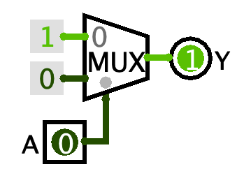
Consider the circuit on the right. It’s a MUX with 1 select bit and 1 Data Bits. The two values going into the data inputs are Wiring > Constants.
- Build it and play with it.
- Make a truth table for it. (That is, list every possible combination of inputs
A, and for each combination of inputs, write down the outputY. Yes it’s going to be a very small truth table.) - What boolean logic operation is this performing? So how could you remake this circuit in a simpler way?
The truth table looks like:
| A | Y |
|---|---|
| 0 | 1 |
| 1 | 0 |
This is logical NOT. So you could replace the whole mux and constants with just a single NOT gate. Sometimes I see students making this big complicated MUX contraption and all it’s doing is a NOT, so now you know to avoid making this!
Now see if you can make a MUX act as an AND gate, and then as an OR gate. You’ll clearly need a second input for both of them. You do not need any gates to do this. It can be done entirely by connecting the inputs and constants to the two data inputs and one select input of the MUXes.
There are probably lots of ways of doing this, but here are the most straightforward solutions:
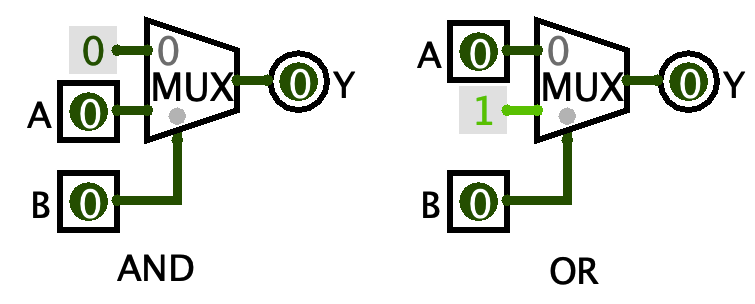
Aren’t they so nice and complementary?
Clocks, dividers, and frequency (Lecture 7)
Let’s explore the clock and blinky circuits a bit.
- Build a circuit like so:
- one Memory > D Flip-flop,
- connect its Q output to a NOT gate
- connect the output of that NOT gate back to its D input
- one Wiring > Clock connected to its clock input
- one Input/Output > LED connected to its Q output as well
- Then, create a second LED and connect the clock signal directly to it.
- Set Simulate > Tick Frequency to 2 Hz, then check Simulate > Ticks Enabled to start the clock.
This circuit is sometimes known as a “blinky,” and it’s kind of the hardware equivalent of “hello, world” - the simplest kind of circuit that shows that everything is working.
Now watch the flashing pattern of the LEDs. How fast does the LED on the clock flash? How fast does the one on the blinky flash?
The clock LED flashes once per second: it’s on for half a second, then off for half a second. But the one connected to the output of the flip-flop is flashing at half that speed: it’s on for a second, then off for a second.
The flip-flop plus NOT gate is actually called a clock divider. This is a circuit that takes an input clock signal, and outputs another clock signal at a slower speed. This is extremely common in digital logic circuits, where often a circuit will have a “master clock” signal which is then divided down to (or multiplied up to) other speeds as needed. The only thing that makes it a “blinky” is the LED :)
Speaking of speed, Hz (Hertz) is the SI unit for frequency. It’s the reciprocal of seconds (s). “2 Hz” means “2 times per second.”
The way Logisim measures clock speed is incorrect: setting it to 2 Hz really makes it run at 1 Hz - 1 FULL clock cycle per second. But at “2 Hz” there are 2 clock edges per second, which is what Logisim is measuring, I guess? This is not the normal way we measure clock speed and I don’t know why Logisim does this.
In the real world, the clock signal is not produced by a little white box with a square wave on it. Instead it’s produced by an oscillator, and there are many different oscillator circuits. An important aspect of real-world clocks is that they tick at a very consistent speed. If the clock speed fluctuated by more than a few fractions of a percent, sequential circuits wouldn’t really work properly.
A popular kind of oscillator is a crystal oscillator, which uses a piezoelectric crystal of quartz to generate a very accurate and stable clock signal, accurate enough that you can make clocks out of it. The kind of clock you hang on your wall, I mean! This is what it means if a clock or watch says “quartz” - it’s using a crystal oscillator to keep time.
- Stop the clock from ticking (either uncheck Simulate > Enable Ticks or just use ctrl/cmd+K to do the same thing).
- Copy and paste your blinky and put the second one to the right of the first.
- On the new blinky’s flip-flop, instead of connecting the clock signal to the triangle input, instead connect the Q output of the first blinky’s flip-flop to the triangle input. Like this:
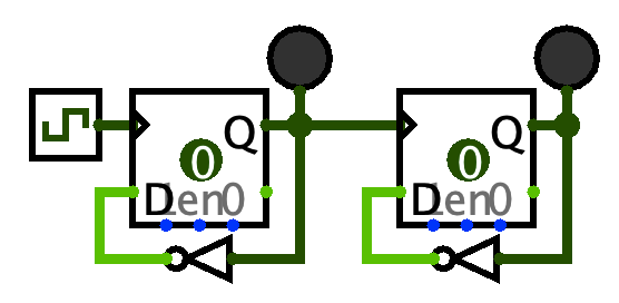
Predict what will happen when you run the clock again. How fast will the LED on the new blinky flash?
It flashes at 1/4 the speed of the original clock. The first divider divides by 2, and then its output becomes the clock signal for the second divider, which divides by 2 again.
You have just made a two-stage clock divider. If you keep copying and pasting, you can make as many stages as you like.
The crystal oscillators found in wall clocks and watches almost universally vibrate at 32,768 Hz. That’s a familiar number, huh. How many divide-by-2 stages would you need to convert the 32,768 Hz from the crystal into a 1 Hz signal to make a wall clock tick?
15 stages. 32,768 = 215, so we have to divide by 215 to get to 1. And this is exactly what’s in every quartz clock - a little chip that has a 15-stage clock divider with the crystal as the input and the second hand as the output. Basically.
Finally, make a three-stage divider (three flip-flops), and include the LED on the clock signal like this:
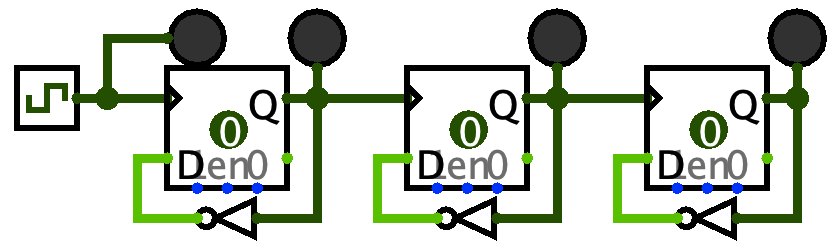
Then start the ticks. Do you notice any pattern that all four lights make? (Hint: try looking at it in a mirror, and remember that on = 1 and off = 0.)
The lights are counting down in binary. The clock is the 1s place, the output of the first stage is the 2s, the output of the second stage is the 4s, etc. That’s why I said “try looking at it in a mirror” - that will put the 8s place on the left and the 1s place on the right.
When you reset (ctrl/cmd+R), it starts off as 0000. The first clock tick takes it to 1111 (15). Then the next takes it to 1110 (14), then 1101 (13), and so on. So apparently this circuit is a clock divider AND a counter! In fact there are commonly-used chips that act as counters or clock dividers depending on how you configure them, like the 74LS68.
State transition diagrams and tables (Lecture 8)
Below is an FSM’s state transition diagram. Answer the questions after it.
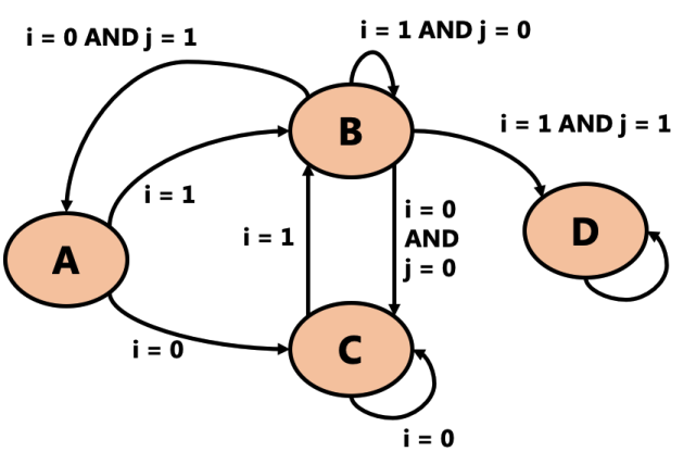
- How many bits would it take to represent the state of this FSM?
- (Count how many states there are, and ask yourself, “what’s the smallest power of 2 that is >= that number?”)
- Once this machine enters state D, it can never go to any other state. Can you think of a situation where it might be useful for a machine to do this?
- What would the state transition table for this machine look like? Hints:
- The table will have 3 input columns (Sn, i, and j) and 1 output column (Sn+1)
- There are as many rows in the table as there are arrows in the diagram
- If the arrow says
ANDfor two inputs, it’s just one row (go look at the example from the slides) - If the arrow doesn’t list a value for an input, then you can put X (“don’t care”) for that input on that row
- The arrow with nothing on it is just missing two inputs, right?
- 2 bits.
- There are 4 states (A, B, C, D), and the smallest power of 2 that can represent that is 22 = 4.
- This could really be anything, but some ideas:
- Maybe this is an FSM that is run when some machine first turns on, and it initializes something and then stops running until the next time you turn it on.
- Maybe D is an “error” state which means something really bad happened and we don’t want to ever continue.
- Or maybe this machine is looking for some pattern of inputs, and D is a “success” state which means it saw that pattern at least once.
- If you ever learned about regular expressions (or in the future, you learn about them), this is a very normal thing to do!
-
The order of the rows doesn’t matter but your table should have all the same rows. Note that the last row is that arrow with nothing on it - so it “doesn’t care” about either input, and always goes back to D.
Sn i j Sn+1 A 0 X C A 1 X B B 0 0 C B 0 1 A B 1 0 B B 1 1 D C 0 X C C 1 X B D X X D
⚠️⚠️⚠️⚠️⚠️⚠️⚠️⚠️⚠️⚠️⚠️⚠️⚠️⚠️⚠️⚠️
This rest page still uses the old ordering of lectures. I haven’t updated it yet.
⚠️⚠️⚠️⚠️⚠️⚠️⚠️⚠️⚠️⚠️⚠️⚠️⚠️⚠️⚠️⚠️
Registers 1 (Lecture 4)
Set t0 and t1 both to the value 100, but you can only use li once.
move copies values between registers.
.global main
main:
    li   t0, 100
    move t1, t0
Registers 2 (Lecture 4)
Show two different ways you could put the value 0 into register t0. (They will be different instructions.)
The zero register is always 0.
.global main
main:
    li   t0, 0
    move t0, zero # does the same thing, but with more typing!
Printing (Lab 1)
Set t0 to 12, then print out its contents with syscall 1. (Remember, t0 is not an argument register. They’re called arguments, not targuments.)
When you want to print the value of a register, you must move its value into a0. Otherwise, the syscall will never see the argument. You aren’t REQUIRED to use move to put the value in a0 for all print syscalls. It’s just that in this case, the value I want to print happens to be in another register, so I must move it. (In other cases I might use lw to load a variable’s contents into a0, or li a value directly into a0. Don’t overfit patterns!)
.global main
main:
    # t0 = 12
    li t0, 12

    # print(t0)
    move a0, t0
    li   v0, 1
    syscall
Math 1 (Lecture 4, Lab 1)
Do the following:
- Set
t0to 30 - Set
t1to 50 - print out the result of doing
t0 * t0 / (t1 + 10), without changingt0ort1. It should print 15.- Remember: PEMDAS…
- also try to use as few registers as possible and as few instructions as possible.
- keep in mind that for printing, you want the value to be printed to end up in
a0.
- keep in mind that for printing, you want the value to be printed to end up in
There are many possible registers that could be used to hold the intermediates. My reasoning:
- since I want to keep
t0andt1unchanged,t2is the next available temp register a0is where I want the result to end up in so I can print it, so why not use it?- I could have used
t3and thenmove a0, t3, but that just adds an extra unnecessary step.
- I could have used
- Fewer registers = less stuff for you to remember = easier to understand.
.global main
main:
    li t0, 30
    li t1, 50

    # PEMDAS says add (parentheses) first, then multiply, then divide

    # remember: you can use constants as the last operand of math instructions!
    add t2, t1, 10  # t2 = (t1 + 10)
    mul a0, t0, t0  # a0 = t0 * t0
    div a0, a0, t2  # a0 = t0 * t0 / (t1 + 10)

    # aaaand print it
    li v0, 1
    syscall
Math 2 (Lecture 4, Lab 1)
Do the following:
- set
t0to 25 - print out the result of doing
1000 / (50 - t0), without changingt0. It should print 40.- see if you can do this using only one more temporary (
t) register.
- see if you can do this using only one more temporary (
This one is a little trickier, because you cannot use constants as the second operand to math instructions, and neither operation is commutative. So, the constants have to be put into a temporary register before each operation.
Notice I used t1 for both constants. You don’t have to keep the constant 50 in t1 after the sub, so don’t worry about reusing the register for another purpose. Hands, not variables.
.global main
main:
    li t0, 25

    # a0 = 50 - t0
    li  t1, 50
    sub a0, t1, t0

    # a0 = 1000 / (50 - t0)
    li t1, 1000
    div a0, t1, a0

    # aaaand print it
    li v0, 1
    syscall
User input (Lab 1)
Syscall 5 works a bit like Scanner.nextInt() in Java. It waits for the user to type an integer and hit enter, and returns that integer in v0 (because that’s what v0 is for: return values).
Write a program that reads an integer that represents a temperature in degrees Celsius, converts it to degrees Fahrenheit, and prints it out. The formula is F = C * 9 / 5 + 32
To test, if you type in 20, you should get 68 out; 30 should give 86; and -40 should give -40 (it’s the same in both scales!).
If you’ve been doing the other exercises so far, this probably isn’t too challenging. But you may have to retrain your brain to stop seeing v0 as just “the register that chooses the syscall to do.” It’s mainly used for return values.
.global main
main:
    # read an integer...
    li v0, 5
    syscall

    # now, v0 is our temperature Celsius. do the conversion
    # into a0 cause we wanna print it out:
    mul a0, v0, 9
    div a0, a0, 5
    add a0, a0, 32

    # aaaand print it.
    li v0, 1
    syscall
Understanding MIPS code 1 (Lecture 4, Lab 1)
Look at the following pieces of code. For each piece of code, write some Java code that does the same thing as the assembly, but in a way that looks like natural Java code. That is, do not translate each line of MIPS to a line of Java. The equivalent Java will be much shorter.
Your pseudocode should not contain any references to MIPS registers. If you need to, you can create variables in your Java, but be sure to name them something that says what they contain, not just int var or int temp or something.
Last, for the syscalls:
- write
printInt(whatever)for syscall 1 - write
readInt()for syscall 5 - write
printChar(whatever)for syscall 11
    # this can be done in a single line of Java.
    li  a0, 50
    sub a0, a0, 3
    mul a0, a0, 13
    rem a0, a0, 600
    li v0, 1
    syscall
printInt(((50 - 3) * 13) % 600);
If you actually calculated it out and got printInt(11), well… that wasn’t the point lol
    # this can be done in a single line of Java.
    li  v0, 5
    syscall
    mul a0, v0, 10
    li  v0, 1
    syscall
No variables needed. Call readInt(), multiply the return value by 1, then print it out. Order of operations applies to functions too - the call to readInt() happens first because it’s inside the outer set of parentheses.
printInt(readInt() * 10);
Identifying loads and stores in HLL code (Lecture 5)
All variables exist in memory, and therefore the only way the CPU can interact with variables is with loads and stores. Remember that loads get the values of variables (copy from memory into a CPU register) and stores set the values of variables (copy from a CPU register into memory.)
High-level languages (HLLs) hide the loads and stores from you, but they still happen every time you access a variable! If you assign into a variable (like x = ...), that is a store, and any other use of a variable (like x + 10 or f(x)) is a load. Some operations - like increment x++ and decrement x-- - do both a load and a store.
Look at these pieces of HLL code and identify the loads and stores. Write your answers as e.g. load x to mean “we load a value from x” or store y to mean “we store a value into y”. Do not translate this code into MIPS! You’re just identifying loads and stores here. Also, there may be multiple loads and/or stores on one line!
int x = 10;
store x- we are only setting
xhere.load xhere would be harmless, but unnecessary. We don’t care what the old value ofxwas (and since we are initializingx, it doesn’t have an old value).
- we are only setting
print(numUsers); // functions are not variables. just focus on the variable!
load numUsers- we are only getting the value of
numUsershere.store numUsersis incorrect! stores are only used to set or change the value of a variable, and we are NOT changing its value here.
- we are only getting the value of
min = i;
load i,store min- again no need to
load minhere - we are only setting its value. - this is also the order in which they happen - we have to load the value of
ifirst, so that we can store its value intomin. (The order of loads and stores is important when you’re writing code, but if you see a question like this on the exam, order won’t matter.)
- again no need to
currentBest = max(currentBest, candidate);
load currentBest,load candidate,store currentBest- get the values of the variables to pass them as arguments to
max; then store the return value intocurrentBest.
- get the values of the variables to pass them as arguments to
    // line numbers in comments; different answers for each line
    int i = 0;      // 1
    while(i < 10) { // 2
        print(i);   // 3
        i++;        // 4
    }
store iload iload iload i,store i
Hopefully this one is simple for you to understand by now. Also, this is exactly the same as a for loop like this:
    for(int i = 0; i < 10; i++) // lines 1, 2, 4
        print(i);               // line 3
The following examples are more complex than anything you would see on the exam, so you don’t have to worry about encountering them then. I’m showing them because they demonstrate some interesting scenarios.
x = i++;
load i,store i,store x- This is confusing code that you should not write. But if you use an increment/decrement operator inside a line of code, there can be multiple stores on one line!
- Because this is a post-decrement,
xwill be assigned the old value ofi, what it contained before being incremented. So ifiwas 4 before this line of code, then after this line of code,x == 4andi == 5. This is confusing, and is exactly why people say to never do this. - …interestingly, all the “confusing, don’t write this” code has multiple stores in a single line. That’s not a coincidence. Changing the values of things is difficult for us to reason about, and doing multiple changes is even harder to understand. So don’t do it!
    int[] array = new int[10]; // 1.
    array[i] = x;              // 2.
store array- this puts the address of the array object into the local variable named
array. arrayonly holds an address! not the array itself.- this is what reference types really are - variables of reference types hold addresses.
- this puts the address of the array object into the local variable named
load x,load array,load i,store array[i]- whooo, this one is a doozy.
- We have to
load xto get its value. That’s easy. - We have to
load array, to get the address of the array object out of thearrayvariable. Importantly, we’re not storing intoarrayhere. Yes, it’s on the left side of the=, but we’re not changingarray. We’re not making it point to a new array object. We are instead changing an item INSIDEarray. - We have to
load ito get its value. This will be combined with the address we got out ofarrayto get the memory location we ultimately want to store into. - And finally, we have to store the value we loaded out of
xintoarray[i]. Array slots are variables so they can be used in loads and stores too. - The ordering of loads depends on the language and implementation and compiler and other factors. But the store will always be the last thing that happens.
    // yes, there is a variable here!
    System.out.println("Hello!");
load System.outSystem.outis a global variable (or in Java terminology, it’s astaticclass variable).- To call a method on
System.out, we have to load it out of the variable. So that’s why there’s a load here. - Note that we don’t have to
load System, becauseSystemis not a variable - it’s a class name.System.outis the full name of the variable we are accessing.
…….
If you want to get really technical, there are actually a couple more loads happening here. See, the way that virtual method calls work in Java is that the addresses of the methods are kept in an array pointed to by the object. The line of code above is really implemented more like:
t0 = System.out;    // load System.out into a register
t1 = t0.methods[7]; // load t0.methods (an array), then load t0.methods[7] (println)
t1(t0, "Hello!");   // call the method in t1 using t0 as the 'this' argument
The 7 above is just an arbitrary number I picked out of a hat. I have no idea if println is the 7th method in the methods array. But it doesn’t matter. The important bit is that the method code address is indexed out of an array.
You’ll also notice I explicitly passed the object - in t0 - as the first argument to the method. That is the this argument in Java, and it’s implicitly passed to every non-static method. a.method() passes a as the this argument to method. This, along with indexing the method out of an array, is what makes object-oriented programming with virtual methods work!
Global variables 1 (Lecture 5, Lab 1)
Do the following:
- Declare a global
.wordvariablevarinitialized to 5. Don’t forget.dataand.text! - In
main, do the equivalent ofprint(var); that is, print its value.
You use lw to load the value of a variable into a register. Here we’re loading directly into a0 because we’re gonna print its value. You can lw into any register; if you did lw t0, var then move a0, t0, that still works, but it’s more typing and more to think about.
If you tried to use li a0, var or move a0, var, you would get an assembler error, because those instructions copy values from other places, not from memory.
.data
    var: .word 5
.text
.global main
main:
    # print(var)
    lw a0, var
    li v0, 1
    syscall
Global variables 2 (Lecture 5, Lab 1)
Do the following:
- Declare three
.wordvariablesx,y, andz, all initialized to 0. - In
main, do:x = 10y = 20z = x + yprint(z)(should print 30)
Be sure you are actually putting values in the variables and not just in the registers! After running your program, look in the “Data Segment” window with “Hexadecimal Values” off. You should see 10, 20, and 30 in the top-left corner of the “Data Segment” window, if you did things correctly.
As your programs get longer, you really should start breaking up sequences of instructions with whitespace and comments saying what the next few instructions do.
Also notice that I used as few registers as possible. t0 is a workhorse, being used in a majority of instructions. It’s my “right hand.” t1 gets some use too, when we want to pick up the values of two variables and add them together.
.data
    x: .word 0
    y: .word 0
    z: .word 0
.text
.global main
main:
    # x = 10
    li t0, 10
    sw t0, x

    # y = 20
    li t0, 20
    sw t0, y

    # z = x + y
    lw  t0, x
    lw  t1, y
    add t0, t0, t1
    sw  t0, z # it's really common to forget to store the value back!

    # print(z)
    # yes, I just stored the value of z in the last instruction. but
    # it's just easier for my brain to reload it with "lw" here.
    lw  a0, z
    li  v0, 1
    syscall
Understanding MIPS code 2 (Lecture 5)
Look at the following pieces of code. For each piece of code, write some Java code that does the same thing as the assembly, but in a way that looks like natural Java code. That is, do not translate each line of MIPS to a line of Java. The equivalent Java will be much shorter.
Your pseudocode should not contain any references to MIPS registers. If you need to, you can create variables in your Java, but be sure to name them something that says what they contain, not just int var or int temp or something.
Last, for the syscalls:
- write
printInt(whatever)for syscall 1 - write
readInt()for syscall 5 - write
printChar(whatever)for syscall 11
    # this can be done in a single line of Java.
    lw  a0, x
    add a0, a0, 1
    li  v0, 1
    syscall
printInt(x + 1);
You are only getting the value of x, not setting it, so x = x + 1 or x++ would be wrong.
    # this can be done in 3 lines of Java.
    li v0, 5
    syscall
    sw v0, width

    li v0, 5
    syscall
    sw v0, height

    lw  t0, width
    lw  t1, height
    mul t0, t0, t1
    sw  t0, area
    width  = readInt();
    height = readInt();
    area   = width * height;
Infinite loops (Lecture 6)
Write an infinite loop that does the equivalent of this, but use a register for the variable i, not a global variable. (Hint: a0 is a poor choice of register. Never use a registers for anything except passing arguments to functions.)
This is an infinite loop, so the program will never stop on its own. You will have to press the stop button at the top of MARS to stop it.
int i = 0;

while(true) {
    System.out.print(i);
    System.out.print('\n'); // syscall 11, remember?
    i++;
}
Infinite loops are made with j (“jump”). Important things about my solution:
- I used a local label name (starts with an underscore) to label the top of the loop.
- All control flow labels should start with an underscore.
- I used
t0as my loop counter register, but really anytregister would be OK here. - I’ve indented the code for clarity as to where the loop begins and ends, but it has no effect on how the code runs.
.global main
main:
    # i = 0
    li t0, 0

    _loop:
        # print(i)
        move a0, t0
        li v0, 1
        syscall

        # print('\n')
        li a0, '\n'
        li v0, 11
        syscall

        # i++
        add t0, t0, 1
    j _loop
If-else (Lecture 6)
Using the print_str macro given in the include file for lab 3, write a program that does the following. The num variable will be a register, not a global.
System.out.print("Number? ");
int num = read_int(); // syscall 5

if((num % 2) == 0) { // % = "rem"
    System.out.print("Even!\n");
} else {
    System.out.print("Odd!\n");
}
- The solution below does not include the definition of the
print_strmacro for brevity. - If you were having trouble with your solution printing “Odd!” for even numbers and “Even!” for odd numbers, you may have forgotten to invert the condition. See how I’m using
bneto choose when to go to theelse. - If your program printed both “Even!” and “Odd!”, you forgot the jump to the
_endiflabel. - I’ve indented the code inside the
if-elsefor clarity, but again it has no effect on how it runs.
.global main
main:
    print_str "Number? "

    # num = read_int()
    li v0, 5
    syscall

    # if((num % 2) == 0)...
    rem t0, v0, 2
    bne t0, 0, _else # "bne t0, zero, _else" works too
        print_str "Even!\n"
    j _endif
    _else:
        print_str "Odd!\n"
    _endif:
Control flow mistakes (Lecture 6)
What is wrong with each piece of code? The comments explain what it should do, but the code doesn’t do that.
This code always prints the message, even if v0 is not 10.
    # if(v0 == 10), print "yay!". otherwise, do nothing.
    beq v0, 10, _print_message
_print_message:
    print_str "yay!\n"
Branching or jumping to the next line of code does absolutely nothing. If v0 is 10, the beq will go to _print_message; and if v0 is not 10, it will still go to _print_message because it’s the next thing after the beq. The beq should be a bne, and it should branch to the line after the print_str, not before it.
When v0 is 1, it prints all the messages in order.
    # switch(v0), and print one of three messages based on its value.
    beq v0, 1, _case1
    beq v0, 2, _case2
    j _default
_case1:
    print_str "it's one!\n"
_case2:
    print_str "it's two!\n"
_default:
    print_str "it's some other value...\n"
Just like in Java, each case needs to end with something like a break. Otherwise, it will fall through the labels and run all the cases after the selected one. There should be a j _break at the end of each case, and a _break: label after the end of the default case.
for loops and arrays (Lecture 7)
Declare an array named constants. It is of type .double and its values are 1.41421, 2.71828, and 3.14159.
Now, in main write a for loop that loops over this array and prints its contents, separated by newlines. Useful info:
- The array length is 3.
- A
.doubleis 8 bytes in size. - To print a double, you must load it using the
l.dinstruction into thef12register, then use syscall 3.- Yes, seriously,
l.d, with a period in it! It works just likelwdoes for.words. - On the right side of MARS, click the “Coproc 1” tab to see the floating-point registers.
- Yes, seriously,
- Use syscall 11 to print a newline (
'\n') after each number.
The output should look like:
1.41421
2.71828
3.14159
Despite using some weird stuff that we otherwise won’t use (.double, the float registers, l.d, syscall 3), this is not really that different from a loop over an array of ints.
I used t0 as the loop counter but you’re not required to. Any t register would have been fine.
.data
    constants: .double 1.41421, 2.71828, 3.14159
.text
.global main
main:
    li t0, 0
    _loop:
        mul t1, t0, 8
        l.d f12, constants(t1)
        li v0, 3
        syscall

        li a0, '\n'
        li v0, 11
        syscall
    add t0, t0, 1
    blt t0, 3, _loop # you can use constants in branches.
Understanding MIPS code 3 (Lectures 6 and 7)
Look at the following pieces of code. For each piece of code, write some Java code that does the same thing as the assembly, but in a way that looks like natural Java code. That is, do not translate each line of MIPS to a line of Java. The equivalent Java will be much shorter.
Your pseudocode should not contain any references to MIPS registers. If you need to, you can create variables in your Java, but be sure to name them something that says what they contain, not just int var or int temp or something.
Last, for the syscalls:
- write
printInt(whatever)for syscall 1 - write
readInt()for syscall 5 - write
printChar(whatever)for syscall 11 - write
print("message")for theprint_str "message"macro.
    # this can be done in two lines of Java.
    lw t0, width
    ble t0, MAX_WIDTH, _L1
        print_str "too wide!\n"
    _L1: # this is a bad label name but I'm trying to hide what this is lol
    if(width > MAX_WIDTH)
        print("too wide!\n");
The if condition in Java is the opposite of what it is in MIPS, because in MIPS, you are checking when to skip the code inside the if, and in Java, you are checking when to run the code inside the if.
By the way, it’s not called an “if loop.” It’s not a loop. It’s just an “if statement” or “an if”.
    # this can be done in two lines of Java. really.
    # remember, write it naturally, not literally.
    li t0, 0
    _L1:
        move a0, t0
        li v0, 1
        syscall
        print_str " "
    add t0, t0, 1
    blt t0, 50, _L1
    for(int i = 0; i < 50; i++)
        System.out.print(i + " ");
It’s okay to take some liberties with the pseudocode to make it more natural. There’s no mention of a variable i in the MIPS, but that’s typically what you name for loop counter variables! Also, in Java you’d probably print the int and the space on a single line with string concatenation, rather than doing two print calls in a row.
    # this can be done in 4 lines of Java.
    lw t0, counter
    beq t0, 0, _L1
        sub t0, t0, 1
        sw  t0, counter
    j _L2
    _L1:
        li  t0, RESET_VALUE
        sw  t0, counter
    _L2:
    if(counter != 0)
        counter--;
    else
        counter = RESET_VALUE;
No variable needed here, even though the MIPS does some funny stuff by breaking up the decrement into a lw before the beq and then a sub-sw after it. The meaning of the Java code is the same, even if it doesn’t do the exact same steps as the original MIPS.
Endianness (Lecture 7)
If you are unsure what endianness your computer is, you can write a program to test it:
- Make a word-sized variable initialized to a 8-digit hexadecimal value that’s different on the two ends.
- e.g.
0xBEEFC0DEor0xDEADBEEFor0xCAFEFACEor even0x11223344if you’re boring
- e.g.
- Use the
lbuinstruction to load the first byte of that variable.lbuis the “unsigned” flavor oflb.- and don’t worry, the computer won’t care if you use
lbuon a.wordvariable. it doesn’t know! the next exercise goes into this in more depth.
- Use syscall 34 to print the value that you loaded.
- this prints an int in hexadecimal instead of decimal.
Look at the output. Which end of the original value is it? That’s what endianness it is. e.g. if you used 0xBEEFC0DE:
- an output of
0x000000bemeans it’s big-endian - an output of
0x000000demeans it’s little-endian
Solution:
.data
    var: .word 0xBEEFC0DE
.text
.global main
main:
    lbu a0, var # loads the first byte of var, whichever end that happens to be
    li  v0, 34
    syscall
Why does this work?
var is at address 0x10010000 (check the labels window when you assemble). 0xBEEFC0DE is 4 bytes long in memory. If the CPU is big-endian, then the byte at 0x10010000 will be the “big end” of the number - so it will be 0xBE. But unless you’re running MARS on a really strange computer, it’s probably little-endian, so the bytes will be in this order:
- address
0x10010000holds0xDE - address
0x10010001holds0xC0 - address
0x10010002holds0xEF - address
0x10010003holds0xBE
So, when we do lbu a0, var, it will load the byte at 0x10010000 - which is 0xDE.
How the assembler assigns memory addresses to labels (Lecture 7)
The .data segment of memory - which contains all our global variables and arrays - starts by default at 0x10010000 in MARS. (This is not universal, it’s just the convention that MARS uses.)
Every time you declare a variable, the assembler:
- makes sure the address it starts at is aligned (a multiple of the byte size of the value)
- reserves the next n bytes in memory for that variable, so that the next variable will not overlap it
It does this from the top of the program to the bottom, keeping track of the next available free location in the .data segment.
Knowing this, see if you can predict what the addresses of these variables will be, before assembling to check in the Labels window (make sure Settings > Show Labels Window is checked ✔️):
.data
    x: .word 10
    y: .word 20
    z: .word 30
.text
The assembler places the variables at these locations:
xat0x10010000(the first location in the.datasegment)yat0x10010004(xwas a.word, which is 4 bytes, so the next available spot is0x10010004)zat0x10010008(same reason as above)
Importantly the addresses are measured in bytes, not bits. So y does not end up at 0x10010020 (0x20 = 32 in base 10), but instead 4 bytes after the start of x.
Also recall that the address of a multi-byte value is the address of its first byte. So for x, its address is 0x10010000, and since it is a .word, that means it also covers 0x10010001 through 0x10010003, but that is left implied.
How about these variables? (How many bytes is one .byte?)
.data
    a: .byte 5
    b: .byte 10
    c: .byte 15
.text
One .byte is 1 byte. 🙃
So the assembler places them at these addresses:
aat0x10010000bat0x10010001cat0x10010002
Since each variable only takes up 1 byte, the “next available address” just increments by 1 for each declaration.
If you got different addresses, maybe you still have the other variables from the previous example? Delete those so that a, b, c are the only variables in the program.
Here’s a more difficult one. Things to ask yourself when making your predictions:
- how many bytes is each variable?
- therefore, what must be true about its address? (what’s that rule called?)
.data
    b: .byte 5
    w: .word 1000
.text
The assembler places them at these addresses:
bat0x10010000wat0x10010004!
You may have expected w to end up at 0x10010001, since it’s after a .byte variable. But no: because of alignment, a .word variable must be at an address that is a multiple of 4. So, the assembler skips ahead by 3 bytes and places w at 0x10010004 instead.
This is really what the .byte and .word commands do: they tell the assembler the alignment and size of each variable. As you will learn in the next exercise, they are not really “types” of the variables.
Using wrong “flavors” of load or store (Lecture 7)
I said that assembly has no types, but then I also said that when you declare variables, you have to “give them a type,” like this:
.data
    big: .word 10000
    little: .byte 10
.text
So which is it? Do variables in assembly have types or not? Well types aren’t just about saying “what kind of value” something is. An important part of types in languages like Java is that the language doesn’t let you do “wrong things” with a type. And that’s really what assembly is missing.
Make a program where you declare the two variables above, in that order. Then in main, print the contents of big. The program should print 10000. (Code to do this is in the button below, but try to do it yourself and use the button to check your work, okay?)
main:
    # print(big)
    lw a0, big
    li v0, 1
    syscall
If we now change the line lw a0, big to lw a0, little, we are using the wrong kind of load for the little variable. We should be using lb or lbu! So…
- Do you think the assembler will give an error about this? Why or why not?
- Do you think the CPU will give an error about this when you run it? Why or why not?
- What actually happens? Why? Think about what the
lwinstruction really does.
- No, the assembler does not give an error about this, because there is no enforcement of type correctness. When you declare the variable as
.byte, all that means is “make enough room in memory for a 1 byte variable.”- If you said “yes”, you’re thinking like a Java programmer! Which isn’t a bad thing. But it’s important to realize that there are no guard rails here. Nothing is stopping you from making this mistake.
- Maybe the CPU will give an error for this. But it will not give a type error.
- The CPU doesn’t know anything about types, or your variables’ names, or anything.
- It could give an error, if
little’s address happened to be a number that is not a multiple of 4. But that’s an alignment error. - But…
- What actually happens is it prints 10.
- We happened to get lucky here. But there’s a big difference between lucky and correct!
- We got lucky that:
little’s address happens to be a multiple of 4, solwdidn’t crash about alignment, and- the bytes after
littleall happen to be 0s.
- Remember that
lwpicks up 4 consecutive bytes of memory, glues them together, and puts the resulting 32-bit value into a register. That’s all it’s doing here. It’s just that those 4 bytes starting at the address oflittlehappen to be:
| 0A | 00 | 00 | 00 |and on a little-endian machine like yours, that gets glued together into
0x0000000A(decimal 10).
Based on the answer to 3 above, think about what might happen if I changed the variables like this; then try it and see what happens, still using the “wrong” lw a0, little code.
    big: .word 10000
    little: .byte 10
    another: .byte 1
This time, the program prints 266. That’s 256 + 10. Why? Because this time, the memory starting at little looks like this:
| 0A | 01 | 00 | 00 |
So when lw glues those bytes together, it gets 0x0000010A (decimal 266).
Try to make this program crash with an alignment error by only changing the order that you declare the variables. Leave the code in main alone. Why does this crash happen?
If I reorder the variables like so:
    big: .word 10000
    another: .byte 1
    little: .byte 10
Now trying to do lw a0, little crashes with an alignment error. This is happening because the assembler assigns the address 0x10010005 to little. That isn’t a multiple of 4, so when you try to lw from it, lw crashes. Hey, at least the CPU sometimes tells you something is wrong! Just not most of the time…
Play around with this program some more. For example:
- Try using
lborlbuonbigand print that out. Why do you get the numbers you get? - What about using
lhorlhuonbig? - What if you put a negative number in
little, like -10, and uselbuon it? Why do you get that number?
lb/lbuwill just pick up the “first” byte ofbig, sign- or zero-extend it, and put that ina0.- decimal 10000 is
0x2710, and since your computer is almost certainly little-endian, the “first” byte is0x10(decimal 16), so that’s what it will print.
- decimal 10000 is
lh/lhupick up the first two bytes ofbig, sign- or zero-extend it, and put that in a0.- Since
0x2710is only 2 bytes, this will seem to work properly and print 10000. - However, it only “works” because the value is small enough to fit in the range of a 16-bit integer.
- If
bigheld a bigger value (like 100000), it would get truncated in a similar way to usinglb/lbu.
- Since
- Depends on the number, but if you did put -10 in
littleand usedlbu, you would get 246.- This is because -10 signed is the exact same bit pattern as 246 unsigned:
11110110binary. - The choice of load instruction -
lbvslbu- is what interprets the number differently. lbwould sign-extend it to 32 bits, andlbuzero-extends it to 32 bits, giving different values in this case.
- This is because -10 signed is the exact same bit pattern as 246 unsigned:
Indexing an array out of bounds (Lecture 7)
In Java, if you index an array out of bounds, you get, well, an ArrayIndexOutOfBoundsException. But I think you may be noticing a pattern about what assembly and the CPU let you do. (That is: basically anything.)
So what happens if you try to index an array out of bounds in assembly? The answer to this also applies to C, if you are in 449!
Declare an array and a variable like this:
.data
    arr: .word 1, 2, 3, 4, 5
    var: .word 42
.text
Now in main, write some code to print out arr[5]. This array is 5 items long, so index 5 should be invalid.
- What does it do instead of crashing?
- Can you explain that based on how memory is laid out in this program? (Hint: look at the labels window and data segment view after assembling. Where do
arrandvarend up in memory?) - What do you think Java does in order to prevent this and throw that exception?
The code for printing would look something like:
    # print(arr[5])
    li  t0, 5       # t0 is the index
    mul t0, t0, 4   # multiply the index by the size of one item
    lw  a0, arr(t0) # and use it in the parens in the lw
    li  v0, 1
    syscall
- It prints 42, which is the value of
var. -
This happens because
arrandvarare right next to each other in memory. If you look in the data segment view, you’ll see:1 | 2 | 3 | 4 | 5 | 42 |42 - the value of
var- is exactly where index 5 of the array would be, if it were 6 items long. But the CPU doesn’t know that. It just does exactly what you tell it to do.lw a0, arr(t0)takes the address ofarr, addst0to it, and loads a word from there. That’s all it can do. -
Java solves this problem by implicitly checking the index every single time you access an array. That is, if you write
arr[i]in Java, it inserts this right before:if(i < 0 || i >= arr.length) throw new ArrayIndexOutOfBoundsException();This prevents the problem, at the cost of doing these checks on every access, which does cost you a little bit of performance.
Simple functions (Lecture 8)
Declare a global variable named count initialized to 0. Make two functions:
count_upwill incrementcount.count_downwill decrementcount.
Then in main, call count_up and count_down a few times. Finally, print out the value of count. If your program goes into an infinite loop, make sure to exit (syscall 10) at the end of main.
Solution:
The code formatting/styling here is important. Assembly languages do not “have” functions, so it’s up to us to divide up our code visually. I like to use a comment with a horizontal line.
These functions take no arguments and return no values, so the a and v registers are unused.
These are examples of functions with side effects: they change their environment in some way. Global variables are part of the “environment,” because multiple functions can see them. Side effects can be useful, but they also make it harder to reason about what a piece of code does, because now you have to consider the function along with all the things it changes.
.data
    count: .word 0
.text

# --------------------------------------
.global main
main:
    # you can call these as many times as you want.
    jal count_up   # count = 1
    jal count_up   # count = 2
    jal count_up   # count = 3
    jal count_down # count = 2

    # print(count)
    lw a0, count
    li v0, 1
    syscall

    # it's important to exit at the end of main!
    li v0, 10
    syscall

# --------------------------------------
count_up:
    lw  t0, count
    add t0, t0, 1
    sw  t0, count
    jr  ra

# --------------------------------------
count_down:
    lw  t0, count
    sub t0, t0, 1
    sw  t0, count
    jr  ra
Functions with arguments and return values (Lecture 8)
Make a function min which takes two arguments, and returns whichever is smaller.
Then in main, call min and print out the results of calling it with these pairs of values:
- 3 and 5 (should print 3)
- 7 and 2 (should print 2)
- 6 and 6 (should print 6)
Feel free to use the print_str macro that you have used many times to put newlines or spaces or whatever between the values.
The code in main is a bit repetitive, but that’s not really the interesting bit. min compares its two arguments and returns the smaller by putting it in v0, which is the One And Only Valid Register to Return Stuff In.
.global main
main:
    # print(min(3, 5))
    li a0, 3
    li a1, 5
    jal min
    move a0, v0
    li v0, 1
    syscall

    print_str "\n"

    # print(min(7, 2))
    li a0, 7
    li a1, 2
    jal min
    move a0, v0
    li v0, 1
    syscall

    print_str "\n"

    # print(min(6, 6))
    li a0, 6
    li a1, 6
    jal min
    move a0, v0
    li v0, 1
    syscall

    # exit
    li v0, 10
    syscall

# -----------------------------------------------------------
# takes 2 arguments (a0, a1) and returns whichever is smaller
min:
    blt a0, a1, _a0_smaller
        move v0, a1
        j _endif
    _a0_smaller:
        move v0, a0
    _endif:
    jr ra
Understanding MIPS code 4 (Lectures 7 and 8)
Look at the following pieces of code. For each piece of code, write some Java code that does the same thing as the assembly, but in a way that looks like natural Java code. That is, do not translate each line of MIPS to a line of Java. The equivalent Java will be much shorter.
Your pseudocode should not contain any references to MIPS registers. If you need to, you can create variables in your Java, but be sure to name them something that says what they contain, not just int var or int temp or something.
Last, for the syscalls:
- write
printInt(whatever)for syscall 1 - write
readInt()for syscall 5 - write
printChar(whatever)for syscall 11 - write
print("message")for theprint_str "message"macro.
# write a 'static' Java method to do this. the signature (return type
# and argument types) can be entirely determined from the MIPS code.
# argument name(s) are up to you.

get_item:
push ra
    # this code can be done in one line of Java.
    add t0, a0, a1
    lb  v0, arr(t0)
pop ra
jr ra
public static byte get_item(int i, int j) {
    return arr[i + j];
}
Who knows what this is for, but this is what it does. No variable needed to stand in for t0. Registers are not variables, sometimes they just hold intermediate values.
    # this can be done in one line of Java. yes, really.
    lw  t0, current_obj
    lb  a0, obj_x(t0)
    lb  a1, obj_y(t0)
    li  a2, COLOR_GREEN
    jal draw_object
draw_object(obj_x[current_obj], obj_y[current_obj], COLOR_GREEN);
See! One line.
    # this can be done in one line of Java.
    jal ask_user_for_number
    mul v0, v0, 4
    lw  a0, numbers(v0)
    li  v0, 1
    syscall
printInt(numbers[ask_user_for_number()]);
In Java, you don’t have to multiply the index by 4 when accessing an array of ints. You can tell it’s an array of ints in the MIPS code because of lw and multiplying the index by 4.
Calling convention violations (Lecture 9)
Each of these functions is doing something that doesn’t really look like a bug, but violates the calling convention we learned.
- What are the problems?
- How would you fix them?
(line numbers in comments for convenience.)
# ------------------------------------------
# I'm trying to print some_variable, but no matter
# what some_variable contains, it just prints some
# arbitrary value.
print_some_variable:     # 1
    push ra              # 2
                         # 3
    lw t0, some_variable # 4
    li v0, 1             # 5
    syscall              # 6
                         # 7
    pop ra               # 8
    jr ra                # 9
# ------------------------------------------
# The 'if' for KEY_L works fine. but the 'if' for
# KEY_R never triggers. it's almost like it's "forgetting"
# which keys I'm pressing between lines 4 and 11.
check_input:                # 1
    push ra                 # 2
                            # 3
    jal input_get_keys_held # 4
                            # 5
    and t0, v0, KEY_L       # 6
    beq t0, 0, _endif_l     # 7
        jal pressed_left    # 8
    _endif_l:               # 9
                            # 10
    and t0, v0, KEY_R       # 11
    beq t0, 0, _endif_r     # 12
        jal pressed_right   # 13
    _endif_r:               # 14
                            # 15
    pop ra                  # 16
    jr ra                   # 17
# ------------------------------------------
# sometimes, when I call this function, the caller breaks
# in really mysterious ways. like, the caller's 's' registers
# get messed up somehow.
print_array:                            # 1
    push ra                             # 2
                                        # 3
    li s0, 0                            # 4
    _loop:                              # 5
        # print(get_array_item(s0))     # 6
        move a0, s0                     # 7
        jal get_array_item              # 8
        move a0, v0                     # 9
        li v0, 1                        # 10
        syscall                         # 11
                                        # 12
        # print a comma after each item # 13
        print_str ", "                  # 14
    add s0, s0, 1                       # 15
    blt s0, ARRAY_LEN, _loop            # 16
                                        # 17
    print_str "\n"                      # 18
                                        # 19
    pop ra                              # 20
    jr ra                               # 21
print_some_variable- on line 4, it loads the value of the variable into
t0instead ofa0. - To fix this, load into
a0to pass it to the syscall. They’re arguments, not targuments.
- on line 4, it loads the value of the variable into
check_input- it calls
input_get_keys_heldon line 4, which returns a value inv0. - that value is used on lines 6 and 11, in the
ands, but… - on line 8, there is
jal pressed_left. after line 8, you no longer know what is inv0. - So the
andon line 11 is assumingv0still contains the return value frominput_get_keys_held, when it may contain something completely different instead. - To fix this, you could either:
- call
input_get_keys_helda second time before line 11, or - move the return value into an
sregister- (and push/pop that
sregister at the beginning/end of the function).
- (and push/pop that
- call
- it calls
print_array- it looks pretty good, it’s using an
sregister as the loop counter because there’s ajalin the loop, but… - it didn’t
push s0at the beginning andpop s0at the end.- This can cause
print_arrayto mess with its caller’s version ofs0.
- This can cause
- To fix this, just add those
push/poplines.
- it looks pretty good, it’s using an
Extension (Lecture 3)
For each pattern of 4 bits, extend it to 8 bits as an unsigned number, then extend it to 8 bits as a signed number.
0000001110011111
0000- zero-extended (unsigned):
0000 0000 - sign-extended (signed):
0000 0000
- zero-extended (unsigned):
0011- zero-extended (unsigned):
0000 0011 - sign-extended (signed):
0000 0011
- zero-extended (unsigned):
1001- zero-extended (unsigned):
0000 1001 - sign-extended (signed):
1111 1001
- zero-extended (unsigned):
1111- zero-extended (unsigned):
0000 1111 - sign-extended (signed):
1111 1111
- zero-extended (unsigned):
Truncation (Lecture 3)
For each pattern of 8 bits:
- Convert it to unsigned decimal, to see what value you’re starting with
- Truncate it to 4 bits (chop off the upper 4 bits)
- Convert that 4-bit number to unsigned decimal, to see what value you ended up with.
- If you get a different value, try to figure out why you got that value.
Unsigned:
0000 01111000 0001
Now do a similar thing for these patterns, except convert them to signed decimal before/after truncating instead.
0000 01111111 11011110 1111
For the unsigned patterns:
0000 0111- Before: 7
- Truncated:
0111 - After: 7 ✅
1000 0001- Before: 129
- Truncated:
0001(not1000, truncation only gives you the lower (right) bits) - After: 1 ⚠️
- You lost a bit!
- You get this value because
129 % 16 == 1. When you truncate, if the value being truncated is too big, it will wrap around based on the number of values possible in the new size. Since we are truncating to 4 bits, that’s 24 = 16.
For the signed patterns:
0000 0111- Before: +7
- Truncated:
0111 - After: +7 ✅
1111 1101- Before: -3
- Truncated:
1101 - After: -3 ✅
- It seems a little weird that we threw out all those
1sand got the same value… - But negative 2’s complement numbers conceptually have an infinite number of 1s in front of them.
- So, throwing those extra 1s away is no more “harmful” to the value than throwing away 0s in front of a positive number.
- (Something like
1111 0000however would not keep its value when truncated to 4 bits though. You have to keep at least one 1 at the beginning for it to stay negative.)
- It seems a little weird that we threw out all those
1110 1111- Before: -17
- Truncated:
1111 - After: -1 ⚠️
- This one got mangled. Oops.
- One way of interpreting how we got -1 is to consider the number circle. The value -17 means “start at 0, then move left (counterclockwise) 17 locations.” If you do that on the 4-bit signed number circle, that will take you around one full revolution (16 locations), then one more, landing you at -1.
- You could also get something similar with remainder/modulus but that gets into weird territory where people disagree so…
Bit shifting (Lecture 14)
For the following, all inputs/outputs are 8 bits. So when shifting left, the result is truncated back down to 8 bits; and when shifting right, you must insert bits on the left to replace the ones that are shifted off the right. Reminder:
<<is left shift>>is signed or arithmetic right shift>>>is unsigned or logical right shift
What are the results of these shifts, in decimal? For the right shifts, the signed-ness of the result is indicated by which shift operator is used. For the left shifts, the signed-ness either doesn’t matter, or is given to you.
5 << 2(same result for signed or unsigned interpretations.)30 << 4(treat the result as an unsigned integer here)5 << 8(hmm…!)100 >> 2-100 >> 2156 >>> 2
5 << 2 == 20- It’s like multiplying by 22 = 4.
30 << 4 == 224, somehow??- 30 is a 5-bit number, so when you shift left by 4, you get a 9-bit number, 480.
- The truncation chops off the topmost bit, leaving you with a weird result.
- 224 is not arbitrary, it’s 480 % 256. When you chop off bits on the left side of a number, that’s like doing modulo by a power of 2.
5 << 8 == 0… maybe.- So, on paper, you might expect all the bits of 5 to get shifted off the left, leaving you with 0s.
- Some CPUs do exactly this. But not all.
- On some other CPUs, the shift distance is actually interpreted modulo the number of bits in a register.
- So shifting left by 8 here might be the same as shifting by 0, and give you 5! Weird!!
100 >> 2 == 25- It copies the sign bit (0) into the two topmost places, keeping it positive.
-100 >> 2 == -25- Same thing, but negative this time.
156 >>> 2 == 39- This is unsigned right shift, so the input/output are interpreted as unsigned.
- (Did you notice 156 is the same bit pattern as
-100?)
Making masks (Lecture 15)
In class we said “to isolate the lowest n bits of a number, bitwise AND with 2n - 1.” That 2n - 1 value is the mask.
We also saw an easy way of coming up with these masks, that didn’t involve remembering/computing large powers of 2. Look that up, and come up with masks for these numbers of bits. Write the masks in hex.
- 8 bits
- 10 bits
- 17 bits
- 27 bits
Each F is 4 bits; then you put a 1, 3, or 7 in front of it based on how many more bits you need.
0xFF0x3FF0x1FFFF0x7FFFFFF
Binary scientific notation (Lecture 15)
Here are some binary numbers. They are not “in 2’s complement” or anything, they’re just numbers, like if you were a person whose society used base 2 instead of base 10, and you wrote them out on paper.
Put each number into binary scientific notation, writing the exponent like x 2^whatever. For example, +101 would be +1.01 x 2^2.
+1-1001001+0.00001-11100.011+10000000000000-0.000000000000111
+1=+1.0 x 2^0-1001001=-1.001001 x 2^6+0.00001=+1.0 x 2^-5-11100.011=-1.1100011 x 2^4+10000000000000=+1.0 x 2^13-0.000000000000111=-1.11 x 2^-13
Encoding IEEE 754 floats (Lecture 15)
Using the numbers in binary scientific notation from the last exercise, encode each one as a single-precision IEEE 754 floating-point number by giving the binary values for each of the three fields:
- sign (1 bit),
- exponent (8 bits), and
- fraction (23 bits).
Remember that the bias constant for single-precision floats is 127, and so the exponent field is basically treated as an unsigned 8-bit number.
+1.0 x 2^0- sign:
0 - exponent:
0111 1111(= 0 + 127) - fraction:
000 0000 0000 0000 0000 0000(the1before the binary point is not encoded!)
- sign:
-1.001001 x 2^6- sign:
1(negative) - exponent:
1000 0101(= 6 + 127) - fraction:
001 0010 0000 0000 0000 0000(you do NOT flip the bits. floats use sign-magnitude.)
- sign:
+1.0 x 2^-5- sign:
0 - exponent:
0111 1010(= -5 + 127) - fraction:
000 0000 0000 0000 0000 0000
- sign:
-1.1100011 x 2^4- sign:
1 - exponent:
1000 0011(= 4 + 127) - fraction:
110 0011 0000 0000 0000 0000
- sign:
+1.0 x 2^13- sign:
0 - exponent:
1000 1100(= 13 + 127) - fraction:
000 0000 0000 0000 0000 0000
- sign:
-1.11 x 2^-13- sign:
1 - exponent:
0111 0010(= -13 + 127) - fraction:
110 0000 0000 0000 0000 0000
- sign:
Decoding IEEE 754 floats (Lecture 15)
Here are 3 encoded IEEE 754 single-precision floats. The divisions between the fields are marked with |. Decode them by writing their value in binary scientific notation (like you used in the last two exercises).
For the exponent: to encode them in the last exercise, you had to add 127. So to decode them, you will have to do the opposite to recover the original exponent. For example, if the encoded exponent is 0111 1111 (127), the original exponent is 0000 0000 (0).
0 | 1000 1100 | 000 0111 0000 0000 0000 00001 | 1000 0111 | 010 0110 1000 0000 0000 00000 | 0111 1110 | 000 0100 0000 0000 0000 0000
0 | 1000 1100 | 000 0111 0000 0000 0000 0000=+1.0000111 x 2^131000 1100is decimal 140; 140 - 127 = 13.
1 | 1000 0111 | 010 0110 1000 0000 0000 0000=-1.01001101 x 2^80 | 0111 1110 | 000 0100 0000 0000 0000 0000=+1.00001 x 2^-1
Numbers of bits in products (Lecture 17)
Here’s an easy one. How many bits will the product be if I multiply together two numbers of these many bits?
- 8
- 20
- 64
If you multiply together two n-bit numbers, you can get a product with at most 2n bits. So for these bit sizes:
- 16
- 40
- 128
Overflow in multiplication and division (Lecture 18)
This one is more of an exploration, and not something we talked about in class. (No, you will not have to remember this for the exam.)
Try running this program in MARS (with Hexadecimal Values turned on):
    li t0, 0x10000
    mult t0, t0
Recall that mult is the “real” multiplication instruction which multiplies its operands and puts the result in hi and lo.
So after running this, look at what’s in hi and lo.
- What 64-bit number do
hiandlorepresent, in hex? - This number doesn’t fit into only 32 bits (8 hex digits), does it? So how would you detect a 32-bit overflow after running this
multinstruction, assuming you did an unsigned multiplication? (Recall thatmfloandmfhimove the values from thelo/hiregisters into a regular register)
Now let’s think about division, specifically signed division. When we think of division, we think of getting numbers smaller than the input. But believe it or not, it is possible to get an overflow - a number too big to be represented - by doing an integer division. (MIPS’s div instruction will not crash in this case, which is a little unfortunate for demonstrating this, but hey.)
What signed integers, when divided, will give a number that is too big to be represented? Hint: it has to do with the shape of the 2’s complement number line…
Multiplication:
hiandlo, “glued together,” represent0x0000000100000000. Thats a 9-digit hex number, or a 33-bit binary number.- You could detect the overflow by using
mfhito get the high-order 32 bits, and testing if they’re 0. For unsigned multiplications, the upper 32 bits will be 0 if the number is < 33 bits. If they’re non-0, an overflow occurred. (It’s kind of an extension of the rule used for detecting overflow in unsigned addition, except now you can get up to 32 bits of “carry out” instead of just 1.)
Division: If you divide the most negative integer (-2n-1) by -1, you will get a number too big to be represented. E.g. if you are dealing with 4-bit numbers, the most negative integer is -8. -8 / -1 = +8, but there is no +8, because the positives only go up to +7. If you want to see this in action in MARS, put 0x80000000 into a register, and then divide that register by -1. It will stay 0x80000000!
Bitfield specifications (Lecture 21)
For the following two bitfield specifications, for each field determine its:
- position,
- size (in bits),
- and mask (in hex, based on the size).
Spec 1:
+------------+-----+---------------------------+
|15        12|11 10|9                         0| <- bit numbers
+------------+-----+---------------------------+
|     A      |  B  |             C             | <- field names
+------------+-----+---------------------------+
Spec 2:
+---------+-------+-------+-------+-----+----------------------+
|31     27|26   24|23   21|20   18|17 16|15                   0|
+---------+-------+-------+-------+-----+----------------------+
|  opc1   |  r1   |  r2   |  r3   |opc2 |         imm          |
+---------+-------+-------+-------+-----+----------------------+
Spec 1:
A- position = 12
- size = 4 bits
- mask =
0xF
B- position = 10
- size = 2 bits
- mask =
0x3
C- position = 0
- size = 10 bits
- mask =
0x3FF
Spec 2:
opc1- position = 27
- size = 5 bits
- mask =
0x1F
r1- position = 24
- size = 3 bits
- mask =
0x7
r2- position = 21
- size = 3 bits
- mask =
0x7
r3- position = 18
- size = 3 bits
- mask =
0x7
opc2- position = 16
- size = 2 bits
- mask =
0x3
imm- position = 0
- size = 16 bits
- mask =
0xFFFF
Encoding and decoding bitfields (Lecture 21)
Using this specification from the previous exercise:
+------------+-----+---------------------------+
|15        12|11 10|9                         0| <- bit numbers
+------------+-----+---------------------------+
|     A      |  B  |             C             | <- field names
+------------+-----+---------------------------+
and using the field positions/sizes that you already figured out, write some one-line Java methods that will encode and decode values in this bitfield. When I say “one-line,” I mean the code inside the braces will just be one line.
The code doesn’t have to be perfect or even compile; all that matters is the “meat” inside the methods that actually does the encoding and decoding. You’ll need 4 methods:
short encode(int A, int B, int C)- encodeA,B, andCinto a single value and return it.int getA(short encoded)- extract fieldAfromencodedand return it.int getB(short encoded)- extract fieldBfromencodedand return it.int getC(short encoded)- extract fieldCfromencodedand return it.
Something like this. I haven’t even tried compiling this because it doesn’t matter.
    short encode(int A, int B, int C) {
        // here would be a good place to check ranges of A, B, C for validity.
        return (A << 12) | (B << 10) | C; // or (C << 0)
    }

    int getA(short encoded) {
        return (encoded >> 12) & 0xF;
    }

    int getB(short encoded) {
        return (encoded >> 10) & 0x3;
    }

    int getC(short encoded) {
        return encoded & 0x3FF; // or (encoded >> 0) & 0x3FF
    }
Scientific Notation practice (Lecture 22)
Put the following numbers into scientific notation. (Remember, that means one non-zero digit before the decimal point.)
- 134
- 7,400
- 998,230
- 0.1
- 0.0056
- 0.00000000372
- 1.34 x 10²
- 7.4 x 10³
- 9.9823 x 10⁵
- 1.0 x 10⁻¹
- 5.6 x 10⁻³
- 3.72 x 10⁻⁹
From SI Prefixes to Engineering/Scientific Notation (Lecture 22)
For each of the following:
First, convert it to engineering notation (so it will have 1, 2, or 3 digits before the decimal point, and an exponent that is a multiple of 3). This is easy because you just replace the SI prefix with its power-of-10 equivalent.
Then, convert it to scientific notation (1 digit before the decimal point) if it isn’t already. Be careful about the exponent!
Also, your answers must include units.
- 13 ns
- 750 µs
- 66 MHz
- 3.5 GHz
- 13 ns =
- Engineering: 13 x 10-9 s (don’t forget the unit - s)
- Scientific: 1.3 x 10⁻⁸ s (decimal point moves left = add)
- 750 µs =
- Engineering: 750 x 10-6 s
- Scientific: 7.5 x 10⁻⁴ s
- 66 MHz =
- Engineering: 66 x 106 Hz
- Scientific: 6.6 x 10⁷ Hz
- 3.5 GHz =
- Engineering: 3.5 x 10⁹ Hz
- Scientific: (it’s already in scientific notation)
From Engineering/Scientific Notation to SI Prefixes (Lecture 22)
For each of the following:
If it’s not in engineering notation already (i.e. the exponent is not a multiple of 3), put it in engineering notation. (Remember, 0.6 is not valid, but 600.0 is. You must have 1, 2, or 3 nonzero digits in front of the decimal point.)
Then, convert from engineering notation to an SI prefix. This should be easy because the exponent is now a power of 3, so it’s just a matter of remembering which prefix is which power.
Don’t forget the units.
- 0.6 x 10⁹ Hz
- 13.4 x 10⁵ Hz
- 7.18 x 10³ Hz
- 6.8 x 10⁻⁴ s
- 228 x 10-9 s
- 94 x 10-13 s
- 600 x 106 Hz = 600 MHz (NOT 0.6 GHz. That looks kind of weird.)
- 1.34 x 10⁶ Hz = 1.34 MHz (NOT 1340 kHz. That also looks weird.)
- 7.18 x 10³ Hz = 7.18 kHz (it’s already in engineering notation)
- 680 x 10-6 s = 680 µs
- 228 x 10-9 s = 228 ns (it’s already in engineering notation)
- 9.4 x 10⁻¹² s = 9.4 ps
Time and Frequency (Lecture 22)
For each value, if it’s time, convert to frequency; if it’s frequency, convert to time. Remember, they are reciprocals of each other, and the unit of frequency is Hz.
Your answers should be written as “naturally” as possible, using SI prefixes instead of scientific or engineering notation. So, “1.5 x 10⁷ Hz” is not okay; 15 MHz is.
- 500 ps
- 40 ns
- 250 ns
- 800 MHz
- 3 GHz (3 significant digits in your answer is fine)
These answers are written using MathJaX, so if you have something like NoScript in your browser, allow the cloudflare CDN to load MathJaX.js so they will render properly.
- 500 ps = 2 GHz
- \(500 \mathrm{\ ps} = 500 \times 10^{-12} \mathrm{\ s} = 5 \times 10^{-10} \mathrm{\ s}\)
- \(\frac{1}{5 \times 10^{-10} \mathrm{\ s}} = 0.2 \times 10^{10} \mathrm{\ Hz} = 2 \times 10^{9} \mathrm{\ Hz} = 2 \mathrm{\ GHz}\)
- 40 ns = 25 MHz
- \(40 \mathrm{\ ns} = 40 \times 10^{-9} \mathrm{\ s} = 4 \times 10^{-8} \mathrm{\ s}\)
- \(\frac{1}{4 \times 10^{-8} \mathrm{\ s}} = 0.25 \times 10^{8} \mathrm{\ Hz} = 25 \times 10^{6} \mathrm{\ Hz} = 25 \mathrm{\ MHz}\)
- 250 ns = 4 MHz
- \(250 \mathrm{\ ns} = 250 \times 10^{-9} \mathrm{\ s} = 2.5 \times 10^{-7} \mathrm{\ s}\)
- \(\frac{1}{2.5 \times 10^{-7} \mathrm{\ s}} = 0.4 \times 10^{7} \mathrm{\ Hz} = 4 \times 10^{6} \mathrm{\ Hz} = 4 \mathrm{\ MHz}\)
- remember that \(2.5 = \frac{5}{2}\), so the reciprocal is \(\frac{2}{5} = 0.4\).
- Don’t torture yourself with long division when you don’t need it!
- 800 MHz = 1.25 ns
- \(800 \mathrm{\ MHz} = 800 \times 10^{6} \mathrm{\ Hz} = 8 \times 10^{8} \mathrm{\ Hz}\)
- \(\frac{1}{8 \times 10^{8} \mathrm{\ Hz}} = 0.125 \times 10^{-8} \mathrm{\ s} = 1.25 \times 10^{-9} \mathrm{\ s} = 1.25 \mathrm{\ ns}\)
- 3 GHz = 333 ps (it’s 333.3 repeating exactly, but whatever)
- \(3 \mathrm{\ GHz} = 3 \times 10^{9} \mathrm{\ Hz}\)
- \(\frac{1}{3 \times 10^{9} \mathrm{\ Hz}} = 0.333 \times 10^{-9} \mathrm{\ s} = 333 \times 10^{-12} \mathrm{\ s} = 333 \mathrm{\ ps}\)